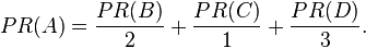
Today i will explain the mathematics behind the Selling Ad Campaigns and Item-to-Item Collaborative Filtering,Search Engine optimization,the concept of crawler and page indexing based to back links to your page so that it comes at the top in the search Engine and can be very promising for your business expansion and sales as more and more people can find it on the search engine. For better advertisement it is necessary that more and more people can find your product and today the best tool that people use to find anything is Google Search Engine so it is very important that your page should be recognized by Google search Engine and it should be given higher significance compared to other related page so that it bubbles up at the top and this procedure of ranking is decided by the back links to your page, means how much links are there who queried about your site ,so higher the back links ie higher the hits on your sight more weight is assigned to your page and hence indexed better and thus better is its rank,So the question is how to put more hits and traffic on the site. Higher traffic will automatically improve the page rank.But how to get more traffic.Know that Google search is based on the Semantics that is the meaningful sentence used by you to describe your content in the Crawlers crawl all through your description of the content and helps in the recognition of your content by search Engine.thus it is very important the you description should be meaningful and words people type in in search engine to find the content information relevant to your page.For Better recognition of your site by search engine use most typed word for that relevant topic. Before knowing this SEO optimization Strategy let's understand different Terminologies and their significance in search strategy Algorithm.
What is Page Rank? Page Rank works by counting the number and quality of links to a page to determine a rough estimate of how important the website is. The underlying assumption is that more important websites are likely to receive more links from other websites and thus increasing the weight of that website so that it bubbles up at the top of search result related to that topic. It is not the only algorithm used by Google to order search engine results, but it is the first algorithm that was used by the company, and it is the best-known. So first step to increase the traffic is to increase the back link shown in the following figure,

So you can see that the website having the highest links coming to it has the highest priority means highest probability to be found by search engine,it is having 38.4% probability to be found by search engine ,higher than the website having lesser number of back links. So in terms of probability we define the occurrence of an event=Finding your website by the search engine in terms of Likelihood of that Event given some condition or prior knowledge base we call that the Baye's rule or conditional probability. so,Mathematical Page Ranks for a simple network, expressed as percentages. (Google uses a logarithmic scale.) Page C has a higher Page Rank than Page E, even though there are fewer links to C; the one link to C comes from an important page and hence is of high value. If web surfers who start on a random page have an 85% likelihood of choosing a random link from the page they are currently visiting, and a 15% likelihood of jumping to a page chosen at random from the entire web, they will reach Page E 8.1% of the time. (The 15% likelihood of jumping to an arbitrary page corresponds to a damping factor of 85%.) Without damping, all web surfers would eventually end up on Pages A, B, or C, and all other pages would have Page Rank zero. In the presence of damping, Page A effectively links to all pages in the web, even though it has no outgoing links of its own.
The Page Rank algorithm outputs a probability distribution used to represent the likelihood that a person randomly clicking on links will arrive at any particular page. PageRank can be calculated for collections of documents of any size. It is assumed in several research papers that the distribution is evenly divided among all documents in the collection at the beginning of the computational process. The Page Rank computations require several passes, called "iterations", through the collection to adjust approximate Page Rank values to more closely reflect the theoretical true value.A probability is expressed as a numeric value between 0 and 1. A 0.5 probability is commonly expressed as a "50% chance" of something happening. Hence, a Page Rank of 0.5 means there is a 50% chance that a person clicking on a random link will be directed to the document with the 0.5 Page Rank.
Simplified Page Rank Algorithm is based upon Set Theory and probability and Each set is a node which represents a web page and its link to other page is represented by an edge thus a page and its link to and from can well be represented by a Graph where you can apply statistical Analysis like Markov process or Bayesian network and Apply Artificial intelligence necessary for a particular Advertisement Requirements.
Let's start as
Assume a small universe of four web pages: A, B, C and D. Links from a page to itself, or multiple outbound links from one single page to another single page, are ignored. Page Rank is initialized to the same value for all pages. In the original form of Page Rank, the sum of Page Rank over all pages was the total number of pages on the web at that time, so each page in this example would have an initial value of 1. However, later versions of Page Rank, and the remainder of this section, assume a probability distribution between 0 and 1. Hence the initial value for each page is 0.25. The Page Rank transferred from a given page to the targets of its outbound links upon the next iteration is divided equally among all outbound links.
If the only links in the system were from pages B, C, and D to A, each link would transfer 0.25 Page Rank to A upon the next iteration, for a total of 0.75.
- Suppose instead that page B had a link to pages C and A, page C had a link to page A, and page D had links to all three pages. Thus, upon the first iteration, page B would transfer half of its existing value, or 0.125, to page A and the other half, or 0.125, to page C. Page C would transfer all of its existing value, 0.25, to the only page it links to, A. Since D had three outbound links, it would transfer one third of its existing value, or approximately 0.083, to A. At the completion of this iteration, page A will have a PageRank of 0.458.
In other words, the PageRank conferred by an outbound link is equal to the document's own PageRank score divided by the number of outbound links L( ).

 ,
,- i.e. the PageRank value for a page u is dependent on the PageRank values for each page v contained in the set Bu (the set containing all pages linking to page u), divided by the number L(v) of links from page v.
Damping factor
The PageRank theory holds that an imaginary surfer who is randomly clicking on links will eventually stop clicking. The probability, at any step, that the person will continue is a damping factor d. Various studies have tested different damping factors, but it is generally assumed that the damping factor will be set around 0.85.
The damping factor is subtracted from 1 (and in some variations of the algorithm, the result is divided by the number of documents (N) in the collection) and this term is then added to the product of the damping factor and the sum of the incoming PageRank scores. That is,


Page and Brin confused the two formulas in their most popular paper "The Anatomy of a Large-Scale Hypertextual Web Search Engine", where they mistakenly claimed that the latter formula formed a probability distribution over web pages
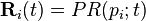
Google recalculates PageRank scores each time it crawls the Web and rebuilds its index. As Google increases the number of documents in its collection, the initial approximation of PageRank decreases for all documents.
The formula uses a model of a random surfer who gets bored after several clicks and switches to a random page. The PageRank value of a page reflects the chance that the random surfer will land on that page by clicking on a link. It can be understood as a Markov chain which i will explain in the following post in which the states are pages, and the transitions, which are all equally probable, are the links between pages.If a page has no links to other pages, it becomes a sink and therefore terminates the random surfing process. If the random surfer arrives at a sink page, it picks another URL at random and continues surfing again.When calculating PageRank, pages with no outbound links are assumed to link out to all other pages in the collection. Their PageRank scores are therefore divided evenly among all other pages. In other words, to be fair with pages that are not sinks, these random transitions are added to all nodes in the Web, with a residual probability usually set to d = 0.85, estimated from the frequency that an average surfer uses his or her browser's bookmark feature.
So, the equation is as follows:

 are the pages under consideration,
  is the set of pages that link to
  ,
,  is the number of outbound links on page
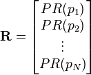
  , and N is the total number of pages.The PageRank values are the entries of the dominant left eigenvector of the modified adjacency matrix. This makes PageRank a particularly elegant metric: the eigenvector is
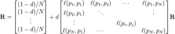
 is 0 if page does not link to , and normalized such that, for each j
 ,
,As a result of Markov theory, it can be shown that the PageRank of a page is the probability of arriving at that page after a large number of clicks. This happens to equal
 where
where  is the expectation of the number of clicks (or random jumps) required to get from the page back to itself.
One main disadvantage of PageRank is that it favors older pages. A new page, even a very good one, will not have many links unless it is part of an existing site (a site being a densely connected set of pages, such as Wikipedia).
Several strategies have been proposed to accelerate the computation of PageRank.
Various strategies to manipulate PageRank have been employed in concerted efforts to improve search results rankings and monetize advertising links. These strategies have severely impacted the reliability of the PageRank concept, which purports to determine which documents are actually highly valued by the Web community.
Since December 2007, when it started actively penalizing sites selling paid text links, Google has combatted link farms and other schemes designed to artificially inflate PageRank.
Computation
PageRank can be computed either iteratively or algebraically. The iterative method can be viewed as the power iteration method or the power method. The basic mathematical operations performed are identical.Iterative
At , an initial probability distribution is assumed, usually
 .
. ,
,
 , (*)
, (*)
 and
and  is the column vector of length
  containing only ones.
The matrix
 is defined as
i.e.,
 ,
, denotes the adjacency matrix of the graph and
  is the diagonal matrix with the outdegrees in the diagonal.
The computation ends when for some small

 ,
,
Algebraic
For (i.e., in the steady state), the above equation (*) reads
 . (**)
 ,
,
 .
.The solution exists and is unique for
 . This can be seen by noting that is by construction a stochastic matrix and hence has an eigenvalue equal to one as a consequence of the Perron–Frobenius theorem.
Power Method
If the matrix is a transition probability, i.e., column-stochastic with no columns consisting of just zeros and  is a probability distribution (i.e.,
  ,
,  where
where  is matrix of all ones), Eq. (**) is equivalent to
 . (***)
is the principal eigenvector of  . A fast and easy way to compute this is using the power method: starting with an arbitrary vector
  , the operator is applied in succession, i.e.,
 ,
,
 .
.
 ,
,
 is an initial probability distribution. In the current case
 .
.
has columns with only zero values, they should be replaced with the initial probability vector . In other words ,
,
 is defined as
 ,
,
 only give the same PageRank if their results are normalized:
HITS algorithm
Hyperlink-Induced Topic Search (HITS; also known as hubs and authorities) is a link analysis algorithm that rates Web pages, developed by Jon Kleinberg. The idea behind Hubs and Authorities stemmed from a particular insight into the creation of web pages when the Internet was originally forming; that is, certain web pages, known as hubs, served as large directories that were not actually authoritative in the information that it held, but were used as compilations of a broad catalog of information that led users directly to other authoritative pages. In other words, a good hub represented a page that pointed to many other pages, and a good authority represented a page that was linked by many different hubs.The scheme therefore assigns two scores for each page: its authority, which estimates the value of the content of the page, and its hub value, which estimates the value of its links to other pages.
Google Search:The main purpose of Google Search is to hunt for text in publicly accessible documents offered by web servers, as opposed to other data, such as images or data contained in databases.
In May 2012 Google introduced a Knowledge Graph semantic search feature in the U.S.
The order of search on Google's search-results pages is based, in part, on a priority rank called a "PageRank". Google Search provides many different options for customized search, using Boolean operators such as: exclusion ("-xx"), alternatives ("xx OR yy OR zz").
Let's discuss the terms defined above to Fully understand Intelligent Search strategy and how you can influence it.
Probability distribution:In probability and statistics, a probability distribution assigns a probability to each measurable subset of the possible outcomes of a random experiment, survey, or procedure of statistical inference. Examples are found in experiments whose sample space is non-numerical, where the distribution would be a categorical distribution; experiments whose sample space is encoded by discrete random variables, where the distribution can be specified by a probability mass function; and experiments with sample spaces encoded by continuous random variables, where the distribution can be specified by a probability density function. More complex experiments, such as those involving stochastic processes defined in continuous time, may demand the use of more general probability measures.
Cumulative distribution function:
Because a probability distribution Pr on the real line is determined by the probability of a scalar random variable X being in a half-open interval (-∞, x], the probability distribution is completely characterized by its cumulative distribution function:
![F(x) = \Pr \left[ X \le x \right] \qquad \text{ for all } x \in \mathbb{R}.](http://upload.wikimedia.org/math/f/4/0/f40b727a379d86fb7cc00b92452ba397.png)
Discrete probability distribution:
A discrete probability distribution should be understood as a probability distribution characterized by a probability mass function. Thus, the distribution of a random variable X is discrete, and X is called a discrete random variable, if
 for n = 1, 2, ..., we have the sum of probabilities 1/2 + 1/4 + 1/8 + ... = 1.
Markov chain:It is a mathematical system that undergoes transitions from one state to another on a state space. It is a random process usually characterized as memoryless: the next state depends only on the current state and not on the sequence of events that preceded it. This specific kind of "memorylessness" is called the Markov property. Markov chains have many applications as statistical models of real-world processes.

Formal definition:A Markov chain is a sequence of random variables X1, X2, X3, ... with the Markov property, namely that, given the present state, the future and past states are independent. Formally,
 . The same information is represented by the transition matrix from time n to time n+1.
However, Markov chains are frequently assumed to be time-homogeneous
(see variations below), in which case the graph and matrix are
independent of n and so are not presented as sequences.
. The same information is represented by the transition matrix from time n to time n+1.
However, Markov chains are frequently assumed to be time-homogeneous
(see variations below), in which case the graph and matrix are
independent of n and so are not presented as sequences.
These descriptions highlight the structure of the Markov chain that is independent of the initial distribution .
When time-homogenous, the chain can be interpreted as a state machine assigning a probability of hopping from each vertex or state to an
adjacent one. The probability
.
When time-homogenous, the chain can be interpreted as a state machine assigning a probability of hopping from each vertex or state to an
adjacent one. The probability  of the machine's state can be analyzed as the statistical behavior of the machine with an element
  of the state space as input, or as the behavior of the machine with the initial distribution
 ![\Pr(X_1=y)=[x_1=y]](http://upload.wikimedia.org/math/2/d/7/2d7f7d08ea5d9a038bad8b2e6e643f38.png) of states as input, where
of states as input, where ![[P]](http://upload.wikimedia.org/math/6/f/5/6f585df5b3729ad672d28b2bd7c5b25d.png) is the Iverson bracket. The stipulation that not all sequences of states must have nonzero probability of occurring allows the graph to have multiple connected components, suppressing edges encoding a 0 transition probability, as if a has a nonzero probability of going to b but a and x lie in different connected components, then
is the Iverson bracket. The stipulation that not all sequences of states must have nonzero probability of occurring allows the graph to have multiple connected components, suppressing edges encoding a 0 transition probability, as if a has a nonzero probability of going to b but a and x lie in different connected components, then  is defined, while
  is not.
 And
And
 , if both conditional probabilities are well defined, i.e. if
  .
.
. The same information is represented by the transition matrix from time n to time n+1.
However, Markov chains are frequently assumed to be time-homogeneous
(see variations below), in which case the graph and matrix are
independent of n and so are not presented as sequences.
These descriptions highlight the structure of the Markov chain that is independent of the initial distribution
.
When time-homogenous, the chain can be interpreted as a state machine assigning a probability of hopping from each vertex or state to an
adjacent one. The probability of the machine's state can be analyzed as the statistical behavior of the machine with an element of the state space as input, or as the behavior of the machine with the initial distribution of states as input, where is the Iverson bracket. The stipulation that not all sequences of states must have nonzero probability of occurring allows the graph to have multiple connected components, suppressing edges encoding a 0 transition probability, as if a has a nonzero probability of going to b but a and x lie in different connected components, then is defined, while is not.Variations:
- Continuous-time Markov processes have a continuous index.
- Time-homogeneous Markov chains (or stationary Markov chains) are processes where

- for all n. The probability of the transition is independent of n.
- A Markov chain of order m (or a Markov chain with memory m), where m is finite, is a process satisfying

- In other words, the future state depends on the past m states. It is possible to construct a chain (Yn) from (Xn) which has the 'classical' Markov property by taking as state space the ordered m-tuples of X values, ie. Yn = (Xn, Xn−1, ..., Xn−m+1).
- The Markov Process :A stochastic process X(t) is said to be a simple Markov process (or first-order Markov) if for any n and a sequence of increasing times t1 < t2 < … < tn , we have
- or equivalently

 If X(t) is a Markov process, then
which means that the process is completely determined by the first-order density function and the conditional density functions. Since the sequence of random variables Xn, Xn – 1, …, X1 is Markov,
E[X n | X n−1 , X n−2 , ... , X1 ] = E[X n | X n−1 ]
Also, the Markov process is Markov in reverse time; that is,

where f(Xn/Xn+1)=Conditional probability density function.
If in a Markov process the present is known, then the past and future are independent; that is, for m < k < n we have


 When the Markov process takes a countable and finite discrete set of values, they are called Markov chains. Markov chains will be developed in more detail in the next page.
MARKOV CHAINS
To master Google Search engine and Statistical predictive model we require to learn Markov Chains.This Model will be very helpful to you to deal with a system showing probabilistic behaviour. we defined the concept of Markov processes above. When the Markov process is discrete-valued (discrete state), it is called a Markov chain. To describe a Markov chain, consider a finite set of states S = {S1 , S2 , ... , S N } .
The process
starts in one of these states and moves successively from one state to another. The move from one state to another is called a step. If the chain is a state Si, it moves to a state Sj in a step with a probability Pij, called transition probability.
The Markov chain is then a discrete state, but may have a discrete or a continuous time. Both cases will be considered in this section.
Discrete-Time Markov Chains
A discrete-time Markov chain must satisfy the following Markov property
 where we have assumed that the random sequence takes a finite, countable set of values. The values of the process are the states of the process, and the conditional probabilities are the transition probabilities between the states, defined in the introduction of this section. If X(n) = i, we say that the chain is in the “ith state at the nth step,” and write
 Since the evolution of the chain is described by the transition probability, when we say that the system is in state j at time tm, given that it is in state i at time tn, we write
 Using Bayes’ rule, we can write
 or, using the new notation
 Assuming that the finite number of states is N, these probabilities must satisfy
 And
And

The total probability is
 In matrix form, the transition matrix or stochastic matrix P (n, m) can be written as

The entries Pij , i, j = 1, 2, K, N, are the transition probabilities that the Markov chain, starting in state Si, will be in state Sj. The initial state matrix is P(0) = P =W , denoted as Π in other books. The column vector
 Hence
Hence

Can be written as
 Homogeneous Chain
A Markov chain is called homogeneous if the transition probabilities depend only on the difference between states; that is,
Pij (m) = P(X n+m = j | X n = i) = P(X m+1 = j | X1 = i)
P(n,m) = P(m− n)
If m = 1,
P(Xn+1 = j | Xn = i) = P(X1 = j | X0 = i) = Pij (1) = Pij
From above equations we can say
P(m) = P(m− n)P(n) = P(m−1)P(1)
where P(1) = P is the one-step transition matrix. Hence, by direct substitution in

We get, P(n,m) = P(m− n)
If m = 1,

Substituting P(n,m) = P(m− n) in P(m) = P(n,m)P(n), we obtain P(m) = P(m− n)P(n) = P(m−1)P(1)
where P(1) = P is the one-step transition matrix. Hence, by direct substitution in
P(m) = P(m− n)P(n) = P(m−1)P(1), we have

We observe that the n-step transition matrix (the matrix of n-step transition probabilities) P(n) is
 Consider the transition matrix P given by
When the Markov process takes a countable and finite discrete set of values, they are called Markov chains. Markov chains will be developed in more detail in the next page. starts in one of these states and moves successively from one state to another. The move from one state to another is called a step. If the chain is a state Si, it moves to a state Sj in a step with a probability Pij, called transition probability.
A Markov chain is called homogeneous if the transition probabilities depend only on the difference between states; that is,
Pij (m) = P(X n+m = j | X n = i) = P(X m+1 = j | X1 = i)
P(Xn+1 = j | Xn = i) = P(X1 = j | X0 = i) = Pij (1) = Pij
P(m) = P(m− n)P(n) = P(m−1)P(1), we have

 State transition diagram
The state transition diagram is shown in Figure above. We see, for example, that the probability in going from state S1 to state S2 is P12 = 0.2, the probability in going from state S2 to state S3 is P23 = 0.5 , and so on.Using
 We have

 As n increases, we reach the situation where the probabilities that the chain is in states S1, S2, and S3 are 0.26, 0.18, and 0.56, respectively, no matter where the chain started. This type of Markov chain is called a regular Markov chain. In general, by definition, if a set of numbers ω1 ,ω2... ,ωN exists, such that
ωi > 0 for all i
We also observe from above example that a homogeneous Markov chain reaches a steady state probability after many transitions. That is,

No comments:
Post a Comment