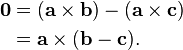
A vector quantity is a quantity that has both a magnitude and a direction and obeys the triangle law of addition or equivalently the parallelogram law of addition. So, a vector is specified by giving its magnitude by a number and its direction. Some physical quantities that are represented by vectors are displacement, velocity, acceleration and force.
Position and Displacement Vectors
The Routing Algorithm is Also based upon finding the shortest path among the given n paths,The light can do it in the space but how can a router choose the shortest path from Ni point Ni+1 when it has M different possibilities.So Router will follow an Algorithm called Dijkstra algorithm which is based upon Triangular inequality.First we will know Dijkstra algorithm and then Mathematics behind this called Triangular inequality that will lead to Artificial intelligence optimal Solution Path.
Djikstra's algorithm (named after its discover, E.W. Dijkstra) solves the problem of finding the shortest path from a point in a graph (the source) to a destination. It turns out that one can find the shortest paths from a given source to all points in a graph in the same time, hence this problem is sometimes called the single-source shortest paths problem.
This problem is related to the spanning tree one. The graph representing all the paths from one vertex to all the others must be a spanning tree - it must include all vertices. There will also be no cycles as a cycle would define more than one path from the selected vertex to at least one other vertex. For a graph,
Dijkstra's algorithm keeps two sets of vertices:
The other data structures needed are:
The basic mode of operation is:
Note that we have also introduced a further way to store a graph (or part of a graph - as this structure can only store a spanning tree), the predecessor sub-graph - the list of predecessors of each node,
pi[j], 1 <= j <= |V|
The edges in the predecessor sub-graph are (pi[v],v).
Now,
The relaxation procedure checks whether the current best estimate of the shortest distance to v (d[v]) can be improved by going through u (i.e. by making u the predecessor of v):
 What is Dijkstra’s Algorithm:
Solution to the single-source shortest path problem in graph theory ! Both directed and undirected graphs ! All edges must have nonnegative weights ! Graph must be connected as shown in the figure below .....

Pseudocode :

Output of Dijkstra’s Algorithm:
Original algorithm outputs value of shortest path not the path itself ! With slight modification you can obtain the path Value: δ(1,6) = 6 Path: {1,2,5,6}
 What is the mathematics behind it that it is working and the answer is Triangular inequality leading to optimal strategy for search Algorithm.
Lemma 1: Optimal Substructure The subpath of any shortest path is itself a shortest path. !
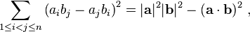
Lemma 2: Triangle inequality If δ(u,v) is the shortest path length between u and v, δ(u,v) ≤ δ(u,x) + δ(x,v) .
Proof of Correctness 1 :
* Invariant: d[v] ≥ δ(s,v) for all v ∈ V
*Holds after initialization and any sequence of relaxation steps
Proof :Hint: We will need the relaxation part of the pseudocode.
d[v] <-- d[u] + w(u,v), Updation will take place iff Triangular inequality Rule.
Proof of Correctness 1.5 :
Relaxation step not only maintains the invariant but allows us to find next shortest path
Suppose s --> ... --> u --> v is a shortest path
* If d[u] = δ(s,u)
*And we relax edge (u,v)
Then d[v] = δ(s,v) after relaxation
Proof
Proof of Correctness 2 :
When Dijkstra terminates,
d[v] = δ(s,v) for all v ∈ V
Proof
Hint: We will need min-extraction part of the pseudocode.
u ← mindistance(Q,dist)

Applications of Dijkstra’s Algorithm:
1)Packet Routing in Data communication Physical layer communication.
2)Light Follow Dijkstra’s Algorithm in free space but it breaks down under intense Gravitational Field.Why?
Algorithms for calculating shortest path from source to sink about as computationally expensive as calculating shortest paths from source to any vertex .
Currency Exchange Problem :
Is there an arbitrage opportunity? ! Ex. $1 # 1.3941 Francs # 0.9308 Euros # $1.00084

Vertex = currency, edge = transaction
! Weight = exchange rate
! Find path that maximizes product of weights # reduce to sum of weights
! Is there a negative cost cycle?

Bellman-Ford Algorithm:
Works for negative weights :
Detects a negative cycle if any exist ! Finds shortest simple path if no negative cycle exists If graph G = (V,E) contains negative-weight cycle, then some shortest paths may not exist.
Come to Actual Greedy Algorithms (Dijkstra’s shortest path algorithm) implementation Step by step you can Apply this Algorithm anywhere where you have to find the shortest path eg Routing a packet through Router Data communication.
Given a graph and a source vertex in graph, find shortest paths from source to all vertices in the given graph.
Dijkstra’s algorithm is very similar to Prim’s algorithm for minimum spanning tree. Like Prim’s MST, we generate a SPT (shortest path tree) with given source as root. We maintain two sets, one set contains vertices included in shortest path tree, other set includes vertices not yet included in shortest path tree. At every step of the algorithm, we find a vertex which is in the other set (set of not yet included) and has minimum distance from source.
Below are the detailed steps used in Dijkstra’s algorithm to find the shortest path from a single source vertex to all other vertices in the given graph.
Algorithm
1) Create a set sptSet (shortest path tree set) that keeps track of vertices included in shortest path tree, i.e., whose minimum distance from source is calculated and finalized. Initially, this set is empty.
2) Assign a distance value to all vertices in the input graph. Initialize all distance values as INFINITE. Assign distance value as 0 for the source vertex so that it is picked first.
3) While sptSet doesn’t include all vertices
….a) Pick a vertex u which is not there in sptSetand has minimum distance value.
….b) Include u to sptSet.
….c) Update distance value of all adjacent vertices of u. To update the distance values, iterate through all adjacent vertices. For every adjacent vertex v, if sum of distance value of u (from source) and weight of edge u-v, is less than the distance value of v, then update the distance value of v.
Let us understand with the following example:

The set sptSetis initially empty and distances assigned to vertices are {0, INF, INF, INF, INF, INF, INF, INF} where INF indicates infinite. Now pick the vertex with minimum distance value. The vertex 0 is picked, include it in sptSet. So sptSet becomes {0}. After including 0 to sptSet, update distance values of its adjacent vertices. Adjacent vertices of 0 are 1 and 7. The distance values of 1 and 7 are updated as 4 and 8. Following subgraph shows vertices and their distance values, only the vertices with finite distance values are shown. The vertices included in SPT are shown in green color.

Pick the vertex with minimum distance value and not already included in SPT (not in sptSET). The vertex 1 is picked and added to sptSet. So sptSet now becomes {0, 1}. Update the distance values of adjacent vertices of 1. The distance value of vertex 2 becomes 12.

Pick the vertex with minimum distance value and not already included in SPT (not in sptSET). Vertex 7 is picked. So sptSet now becomes {0, 1, 7}. Update the distance values of adjacent vertices of 7. The distance value of vertex 6 and 8 becomes finite (15 and 9 respectively).
 Pick the vertex with minimum distance value and not already included in
SPT (not in sptSET). Vertex 6 is picked. So sptSet now becomes {0, 1, 7,
6}. Update the distance values of adjacent vertices of 6. The distance
value of vertex 5 and 8 are updated.
Pick the vertex with minimum distance value and not already included in
SPT (not in sptSET). Vertex 6 is picked. So sptSet now becomes {0, 1, 7,
6}. Update the distance values of adjacent vertices of 6. The distance
value of vertex 5 and 8 are updated.
 We repeat the above steps until sptSet doesn’t include all vertices of given graph. Finally, we get the following Shortest Path Tree (SPT).

Let's code all this Sequence of steps in C++ code as follows
however, is not equal to A because its direction is opposite to that of A We define the negative of a vector as a vector having the same magnitude as the original vector but the opposite direction. The negative of vector quantity A is denoted as -A and we use a boldface minus sign to emphasize the vector nature of the quantities.
We usually represent the magnitude of a vector quantity (in the case of a displacement vector, its length) by the same letter used for the vector, but in light italic type with no arrow on top. An alternative notation is the vector symbol with vertical bars on both sides:
 The magnitude of a vector quantity is a scalar quantity (a number) and is always positive

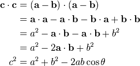
 This triangle law of vector addition is universal it can ve applied to any two non zero vectors to find its resultant sum vector as follows


Position and Displacement Vectors
To describe the position of an object moving in a plane, we need to choose a convenient point, say O as origin. Let P and P′ be the positions of the object at time t and t′ , respectively as shown below
 We join O and P by a straight line. Then, OP is the position vector of the object at time t. An arrow is marked at the head of this line. It is represented by a symbol r, i.e. OP = r. Point P′ is represented by another position vector, OP′ denoted by r′ . The length of the vector r represents the magnitude of the vector and its direction is the direction in which P lies as seen from O. If the object moves from P to P′ , the vector PP′ (with tail at P and tip at P′ ) is called the displacement vector corresponding to motion from point P (at time t) to point P′ (at time t′ ). It is important to note that displacement vector is the straight line joining the initial and final positions and does not depend on the actual path undertaken by the object between the two positions. For example, in Fig b, given the initial and final positions as P and Q, the displacement vector is the same PQ for different paths of journey, say PABCQ, PDQ, and PBEFQ. Therefore, the magnitude of displacement is either less or equal to the path length of an object between two points.
Vectors and Vector Addition :
We start with the simplest of all vector quantities: displacement. Displacement is simply a change in position of an object, which we will assume can be treated as a pointlike particle. In Figure 1.6a, we represent the object’s change in position by an arrow that points from the starting position to the ending position.Displacement is a vector quantity because we must state not only how far the particle
moves, but also in what direction.Walking 3 km north from your front door doesn’t get you to the same place as walking 3 km southeast.We usually represent a vector quantity, such as a displacement, by a single letter, such as A as shown below
 A displacement is always a straight-line segment, directed from the starting
point to the endpoint, even though the actual path of the object may be curved. In
Figure b,the displacement is still A, even though the object takes a roundabout
path. Also, note that displacement is not related directly to the total distance traveled. If the particle makes a round trip, returning to its starting point as shown in Figure c, the displacement for the entire trip is zero.
Displacement is a vector quantity. A displacement vector represents a change in position (distance and direction) of an object from one point in space to another.
Displacement is the Shortest path between any two given points.Light always follow the shortest path Algorithm in free space ie it takes the shortest distance between any given two points.Vectors and Vector Addition :
We start with the simplest of all vector quantities: displacement. Displacement is simply a change in position of an object, which we will assume can be treated as a pointlike particle. In Figure 1.6a, we represent the object’s change in position by an arrow that points from the starting position to the ending position.Displacement is a vector quantity because we must state not only how far the particle
moves, but also in what direction.Walking 3 km north from your front door doesn’t get you to the same place as walking 3 km southeast.We usually represent a vector quantity, such as a displacement, by a single letter, such as A as shown below
point to the endpoint, even though the actual path of the object may be curved. In
Figure b,the displacement is still A, even though the object takes a roundabout
path. Also, note that displacement is not related directly to the total distance traveled. If the particle makes a round trip, returning to its starting point as shown in Figure c, the displacement for the entire trip is zero.
Displacement is a vector quantity. A displacement vector represents a change in position (distance and direction) of an object from one point in space to another.
The Routing Algorithm is Also based upon finding the shortest path among the given n paths,The light can do it in the space but how can a router choose the shortest path from Ni point Ni+1 when it has M different possibilities.So Router will follow an Algorithm called Dijkstra algorithm which is based upon Triangular inequality.First we will know Dijkstra algorithm and then Mathematics behind this called Triangular inequality that will lead to Artificial intelligence optimal Solution Path.
Djikstra's algorithm (named after its discover, E.W. Dijkstra) solves the problem of finding the shortest path from a point in a graph (the source) to a destination. It turns out that one can find the shortest paths from a given source to all points in a graph in the same time, hence this problem is sometimes called the single-source shortest paths problem.
This problem is related to the spanning tree one. The graph representing all the paths from one vertex to all the others must be a spanning tree - it must include all vertices. There will also be no cycles as a cycle would define more than one path from the selected vertex to at least one other vertex. For a graph,
| G = (V,E) | where |
|
| S | the set of vertices whose shortest paths from the source have already been determined and | |
| V-S | the remaining vertices. |
| d | array of best estimates of shortest path to each vertex | |||||
| pi | an array of predecessors for each vertex. |
The basic mode of operation is:
- Initialise d and pi,
- Set S to empty,
- While there are still vertices in V-S,
- Sort the vertices in V-S according to the current best estimate of their distance from the source,
- Add u, the closest vertex in V-S, to S,
- Relax all the vertices still in V-S connected to u
Relaxation
The relaxation process updates the costs of all the vertices, v, connected to a vertex, u, if we could improve the best estimate of the shortest path to v by including (u,v) in the path to v. The relaxation procedure proceeds as follows:initialise_single_source( Graph g, Node s )
for each vertex v in Vertices( g )
g.d[v] := infinity
g.pi[v] := nil
g.d[s] := 0;
This sets up the graph so that each node has no predecessor
(pi[v] = nil) and the estimates of the cost (distance) of
each node from the source (d[v]) are infinite, except for
the source node itself (d[s] = 0). Note that we have also introduced a further way to store a graph (or part of a graph - as this structure can only store a spanning tree), the predecessor sub-graph - the list of predecessors of each node,
Now,
The relaxation procedure checks whether the current best estimate of the shortest distance to v (d[v]) can be improved by going through u (i.e. by making u the predecessor of v):
relax( Node u, Node v, double w[][] )
    if d[v] > d[u] + w[u,v] then
       d[v] := d[u] + w[u,v]
       pi[v] := u
The algorithm itself is now:
shortest_paths( Graph g, Node s )
    initialise_single_source( g, s )
    S := { 0 }        /* Make S empty */
    Q := Vertices( g ) /* Put the vertices in a PQ */
    while not Empty(Q)
        u := ExtractCheapest( Q );
        AddNode( S, u ); /* Add u to S */
        for each vertex v in Adjacent( u )
            relax( u, v, w )
Another Interpretation for above Algorithm which involves more Mathematics is as following
Single-Source Shortest Path Problem:
The problem of finding shortest paths from a source
vertex v to all other vertices in the graph.
! Weighted graph G = (E,V)
! Source vertex s ∈ V to all vertices v ∈ V
Solution to the single-source shortest path problem in graph theory ! Both directed and undirected graphs ! All edges must have nonnegative weights ! Graph must be connected as shown in the figure below .....
Pseudocode :
Output of Dijkstra’s Algorithm:
Original algorithm outputs value of shortest path not the path itself ! With slight modification you can obtain the path Value: δ(1,6) = 6 Path: {1,2,5,6}
Lemma 1: Optimal Substructure The subpath of any shortest path is itself a shortest path. !
Lemma 2: Triangle inequality If δ(u,v) is the shortest path length between u and v, δ(u,v) ≤ δ(u,x) + δ(x,v) .
Proof of Correctness 1 :
* Invariant: d[v] ≥ δ(s,v) for all v ∈ V
*Holds after initialization and any sequence of relaxation steps
Proof :Hint: We will need the relaxation part of the pseudocode.
d[v] <-- d[u] + w(u,v), Updation will take place iff Triangular inequality Rule.
Proof of Correctness 1.5 :
Relaxation step not only maintains the invariant but allows us to find next shortest path
Suppose s --> ... --> u --> v is a shortest path
* If d[u] = δ(s,u)
*And we relax edge (u,v)
Then d[v] = δ(s,v) after relaxation
Proof
Proof of Correctness 2 :
When Dijkstra terminates,
d[v] = δ(s,v) for all v ∈ V
Proof
Hint: We will need min-extraction part of the pseudocode.
u ← mindistance(Q,dist)
Applications of Dijkstra’s Algorithm:
1)Packet Routing in Data communication Physical layer communication.
2)Light Follow Dijkstra’s Algorithm in free space but it breaks down under intense Gravitational Field.Why?
Algorithms for calculating shortest path from source to sink about as computationally expensive as calculating shortest paths from source to any vertex .
Currency Exchange Problem :
Is there an arbitrage opportunity? ! Ex. $1 # 1.3941 Francs # 0.9308 Euros # $1.00084
Vertex = currency, edge = transaction
! Weight = exchange rate
! Find path that maximizes product of weights # reduce to sum of weights
! Is there a negative cost cycle?
Bellman-Ford Algorithm:
Works for negative weights :
Detects a negative cycle if any exist ! Finds shortest simple path if no negative cycle exists If graph G = (V,E) contains negative-weight cycle, then some shortest paths may not exist.
Come to Actual Greedy Algorithms (Dijkstra’s shortest path algorithm) implementation Step by step you can Apply this Algorithm anywhere where you have to find the shortest path eg Routing a packet through Router Data communication.
Given a graph and a source vertex in graph, find shortest paths from source to all vertices in the given graph.
Dijkstra’s algorithm is very similar to Prim’s algorithm for minimum spanning tree. Like Prim’s MST, we generate a SPT (shortest path tree) with given source as root. We maintain two sets, one set contains vertices included in shortest path tree, other set includes vertices not yet included in shortest path tree. At every step of the algorithm, we find a vertex which is in the other set (set of not yet included) and has minimum distance from source.
Below are the detailed steps used in Dijkstra’s algorithm to find the shortest path from a single source vertex to all other vertices in the given graph.
Algorithm
1) Create a set sptSet (shortest path tree set) that keeps track of vertices included in shortest path tree, i.e., whose minimum distance from source is calculated and finalized. Initially, this set is empty.
2) Assign a distance value to all vertices in the input graph. Initialize all distance values as INFINITE. Assign distance value as 0 for the source vertex so that it is picked first.
3) While sptSet doesn’t include all vertices
….a) Pick a vertex u which is not there in sptSetand has minimum distance value.
….b) Include u to sptSet.
….c) Update distance value of all adjacent vertices of u. To update the distance values, iterate through all adjacent vertices. For every adjacent vertex v, if sum of distance value of u (from source) and weight of edge u-v, is less than the distance value of v, then update the distance value of v.
Let us understand with the following example:
The set sptSetis initially empty and distances assigned to vertices are {0, INF, INF, INF, INF, INF, INF, INF} where INF indicates infinite. Now pick the vertex with minimum distance value. The vertex 0 is picked, include it in sptSet. So sptSet becomes {0}. After including 0 to sptSet, update distance values of its adjacent vertices. Adjacent vertices of 0 are 1 and 7. The distance values of 1 and 7 are updated as 4 and 8. Following subgraph shows vertices and their distance values, only the vertices with finite distance values are shown. The vertices included in SPT are shown in green color.
Pick the vertex with minimum distance value and not already included in SPT (not in sptSET). The vertex 1 is picked and added to sptSet. So sptSet now becomes {0, 1}. Update the distance values of adjacent vertices of 1. The distance value of vertex 2 becomes 12.
Pick the vertex with minimum distance value and not already included in SPT (not in sptSET). Vertex 7 is picked. So sptSet now becomes {0, 1, 7}. Update the distance values of adjacent vertices of 7. The distance value of vertex 6 and 8 becomes finite (15 and 9 respectively).
Let's code all this Sequence of steps in C++ code as follows
// A C / C++ program for Dijkstra's single source shortest path algorithm.// The program is for adjacency matrix representation of the graph#include <stdio.h>#include <limits.h>// Number of vertices in the graph#define V 9// A utility function to find the vertex with minimum distance value, from// the set of vertices not yet included in shortest path treeint minDistance(int dist[], bool sptSet[]){ // Initialize min value int min = INT_MAX, min_index; for (int v = 0; v < V; v++) if (sptSet[v] == false && dist[v] <= min) min = dist[v], min_index = v; return min_index;}// A utility function to print the constructed distance arrayint printSolution(int dist[], int n){ printf("Vertex Distance from Source\n"); for (int i = 0; i < V; i++) printf("%d \t\t %d\n", i, dist[i]);}// Funtion that implements Dijkstra's single source shortest path algorithm// for a graph represented using adjacency matrix representationvoid dijkstra(int graph[V][V], int src){ int dist[V]; // The output array. dist[i] will hold the shortest // distance from src to i bool sptSet[V]; // sptSet[i] will true if vertex i is included in shortest // path tree or shortest distance from src to i is finalized // Initialize all distances as INFINITE and stpSet[] as false for (int i = 0; i < V; i++) dist[i] = INT_MAX, sptSet[i] = false; // Distance of source vertex from itself is always 0 dist[src] = 0; // Find shortest path for all vertices for (int count = 0; count < V-1; count++) { // Pick the minimum distance vertex from the set of vertices not // yet processed. u is always equal to src in first iteration. int u = minDistance(dist, sptSet); // Mark the picked vertex as processed sptSet[u] = true; // Update dist value of the adjacent vertices of the picked vertex. for (int v = 0; v < V; v++) // Update dist[v] only if is not in sptSet, there is an edge from // u to v, and total weight of path from src to v through u is // smaller than current value of dist[v] if (!sptSet[v] && graph[u][v] && dist[u] != INT_MAX && dist[u]+graph[u][v] < dist[v]) dist[v] = dist[u] + graph[u][v]; } // print the constructed distance array printSolution(dist, V);}// driver program to test above functionint main(){ /* Let us create the example graph discussed above */ int graph[V][V] = {{0, 4, 0, 0, 0, 0, 0, 8, 0}, {4, 0, 8, 0, 0, 0, 0, 11, 0}, {0, 8, 0, 7, 0, 4, 0, 0, 2}, {0, 0, 7, 0, 9, 14, 0, 0, 0}, {0, 0, 0, 9, 0, 10, 0, 0, 0}, {0, 0, 4, 0, 10, 0, 2, 0, 0}, {0, 0, 0, 14, 0, 2, 0, 1, 6}, {8, 11, 0, 0, 0, 0, 1, 0, 7}, {0, 0, 2, 0, 0, 0, 6, 7, 0} }; dijkstra(graph, 0); return 0;}
Output:
1) The code calculates shortest distance, but doesn’t calculate the path information. We can create a parent array, update the parent array when distance is updated (like prim’s implementation) and use it show the shortest path from source to different vertices.
2) The code is for undirected graph, same dijekstra function can be used for directed graphs also.
3) The code finds shortest distances from source to all vertices. If we are interested only in shortest distance from source to a single target, we can break the for loop when the picked minimum distance vertex is equal to target (Step 3.a of algorithm).
4) Time Complexity of the implementation is O(V^2). If the input graph is represented using adjacency list, it can be reduced to O(E log V) with the help of binary heap. We will soon be discussing O(E Log V) algorithm as a separate post.
5) Dijkstra’s algorithm doesn’t work for graphs with negative weight edges. For graphs with negative weight edges, Bellman–Ford algorithm can be used, we will soon be discussing it as a separate post.
Please write comments if you find anything incorrect, or you want to share more information about the topic discussed above.
Let's come to physics and see vectors Application in different branches of Science and Technology.First study vectors in the general form then i will talk about its application in different fields.
At this moment you must appreciate that to understand Algorithms you should also have the knowledge of vectors.

Vertex   Distance from Source
0                0
1                4
2                12
3                19
4                21
5                11
6                9
7                8
8                14
Notes:
1) The code calculates shortest distance, but doesn’t calculate the path information. We can create a parent array, update the parent array when distance is updated (like prim’s implementation) and use it show the shortest path from source to different vertices.
2) The code is for undirected graph, same dijekstra function can be used for directed graphs also.
3) The code finds shortest distances from source to all vertices. If we are interested only in shortest distance from source to a single target, we can break the for loop when the picked minimum distance vertex is equal to target (Step 3.a of algorithm).
4) Time Complexity of the implementation is O(V^2). If the input graph is represented using adjacency list, it can be reduced to O(E log V) with the help of binary heap. We will soon be discussing O(E Log V) algorithm as a separate post.
5) Dijkstra’s algorithm doesn’t work for graphs with negative weight edges. For graphs with negative weight edges, Bellman–Ford algorithm can be used, we will soon be discussing it as a separate post.
Please write comments if you find anything incorrect, or you want to share more information about the topic discussed above.
Let's come to physics and see vectors Application in different branches of Science and Technology.First study vectors in the general form then i will talk about its application in different fields.
At this moment you must appreciate that to understand Algorithms you should also have the knowledge of vectors.

however, is not equal to A because its direction is opposite to that of A We define the negative of a vector as a vector having the same magnitude as the original vector but the opposite direction. The negative of vector quantity A is denoted as -A and we use a boldface minus sign to emphasize the vector nature of the quantities.
We usually represent the magnitude of a vector quantity (in the case of a displacement vector, its length) by the same letter used for the vector, but in light italic type with no arrow on top. An alternative notation is the vector symbol with vertical bars on both sides:
The magnitude of a vector quantity is a scalar quantity (a number) and is always positive
Vector Addition and Subtraction
Suppose a particle undergoes a displacement A followed by a second displacement B.The final result is the same as if the particle had started at the same initial
point and undergone a single displacement C as shown below.
point and undergone a single displacement C as shown below.
We call displacement C the vector sum, or resultant, of displacements A and B.
We express this relationshipsymbolically as
C=A+B or
Commutative Law of vector addition.
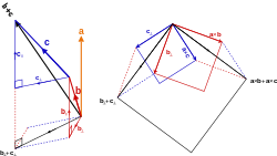
If we combine the above two condition we can derive the parallelogram law of vector addition.
We can also add them by constructing a parallelogram as following.
More details can be found in next paper.
Electronics And Communication by Md Tauseef Ibrahim/Abraham malik click the link here:http://electronicsandcommunicationadvancedma.blogspot.in/2015/03/3g-networksorthogonal-frequency.html
https://t.co/vcjSU1HzdO
y=Cos(x) and Inverse of Cosine as x=arccos(y),but plotted in Cartesian system as X->y &y->X pic.twitter.com/rjL1ctkuvb
— Abraham Malik (@brhmmlk93_malik) March 6, 2015


 (as in the Pythagorean theorem or the Euclidean norm), and
 ,
,


 and
and
 , with
  rotation matrix.
 is a 3-by-3 matrix and
  is the transpose of the inverse. It can be readily seen how this formula reduces to the former one if


![\begin{align}
\ [1, 3, -5] \cdot [4, -2, -1] &= (1)(4) + (3)(-2) + (-5)(-1) \\
&= 4 - 6 + 5 \\
&= 3.
\end{align}](http://upload.wikimedia.org/math/1/3/1/131c946a85f1e689a920763c11f89d5a.png)
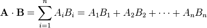
 . The dot product of two Euclidean vectors A and B is defined by


 is the unit vector in the direction of B


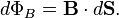


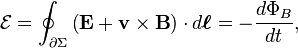
 is the electromotive force (EMF),


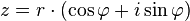 and this can be represented onto polar coordinate system as shown below here


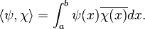
 or the field of complex numbers
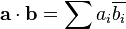
  . It is usually denoted by
  . The inner product of two vectors over the field of complex numbers is, in general, a complex number, and is sesquilinear instead of bilinear. An inner product space is a normed vector space, and the inner product of a vector with itself is real and positive-definite.