Vectors and its application in Physics and Dynamics.
http://t.co/eQSpd40fb2 pic.twitter.com/4k1ThFqOqo
— Abraham Malik (@brhmmlk93_malik) March 4, 2015
Today we will learn vectors and vector Calculus that finds great application in Mechanics and particle dynamics.
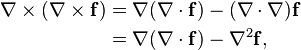
Vector calculus deals with the rate of change of vector with respect to the domain upon which vector depends so if vector depends upon time then rate of change of difference vector with respect to time gives velocity vector means linear combination of velocity along X and Y direction V=Vxi+Vyj=dr/dt,where r=dXi+dYj is the difference vector which we are going to see now.
Before dealing with vector calculus lets deal with vectors in the light of motion in a plane.
Velocity in a Plane:
To describe the motion of an object in a plane, we first need to be able to describe the object’s position Often, it’s useful to use a familiar x-y axis system as shown in the Figure

For example, when a football player kicks a field goal, the ball (represented by point P) moves in a vertical plane. The ball’s
horizontal distance from the origin O at any time is x, and its vertical distance above the ground at any time is y. The numbers x and and y are called the coordinates of point P.The vector r from the origin O to point P is called the position vector of point P, and the Cartesian coordinates x and y of point P are the x and y components, respectively, of vector r.The distance of point P from the origin is the magnitude of vector r
 Where X= r*cos(theta) and Y=r*sin(theta) in polar Coordinate system as shown below
 Converting between polar and Cartesian coordinates:
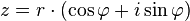
The polar coordinates r and ϕ can be converted to the Cartesian coordinates x and y by using the trigonometric functions sine and cosine:
Let's consider a particle in this polar or Cartesian Coordinate system is at point P1 and moves to P2 as shown in the following figure
 The above figure shows the ball at two points in its curved path.At time t1 it is at a point P1with position vector r1,at the later time t2 it is at the point P2 with position vector r2.The ball moves from Point P1 to P2 during a time interval del t=t2--t1.The change in position (the displacement) during this interval is the vector
 We can relate this difference vector to average velocity simply by dividing this difference vector by the time change required to take place this change.
Let's understand the concept of Average velocity: Above figure in pink shows us that.

So what if we want to find the velocity at a particular instant of time to understand this we require to understand the concept of differential calculus:
The concept of instantaneous velocity and the differential calculus.
To understand instantaneous velocity ie the velocity at a point in the path of motion we require to understand the slope of tangent to the curve at that point .To understand the concept of slope of a tangent to a curve we have to understand Derivative of a function at any poin P(x,y) .And To understand Derivative of a function we require to understand a branch of differential calculus called Limit of a function means approximate value of a function when Domain X-->a, Where a must lie within domain and we write it mathematically as a (-Domain .
We define the instantaneous velocity as follows:
 The two velocity components for motion in the x-y plane


At every point along the path, the instantaneous velocity vector is
tangent to the path.

Because velocity is a vector quantity, we may represent it either in terms of its components or in terms of its magnitude and direction,
The direction of an object’s instantaneous velocity at any point is always tangent to the path at that point. But in general, the position vector r does not have the same direction as the instantaneous velocity v (The direction of the position vector r depends on where you place the origin, while the direction of is determined by the shape of the path.)
Acceleration in a Plane:
Observe the figure given below


Average acceleration is a vector quantity in the same direction as the vector, we stressed that acceleration is a quantitative description of the dv.

 We define the instantaneous acceleration vector(a) at point P1 as shown in the following figure as follows

Again to understand the concept of instantaneous acceleration we require to apply the concept of Limit from differential calculus.
Let's understand instantaneous acceleration:

The instantaneous acceleration vector at point P1 as shown in the above figure does not have the same direction as the instantaneous velocity vector V at that point in general,there is no reason it should. ( The velocity and acceleration components of a particle moving along a line could have opposite signs also.)The construction in above Figure shows that the acceleration vector must always point toward the concave side of the curved path. When a particle moves in a curved path, it always has nonzero acceleration, even when it moves with constant speed. More generally, acceleration is associated with change of speed change of direction of velocity, or both.


We often represent the acceleration of a particle in terms of the components of this vector quantity.


Two special cases a) acceleration parallel to object's velocity
b)acceleration orthogonal to object's velocity


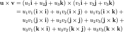
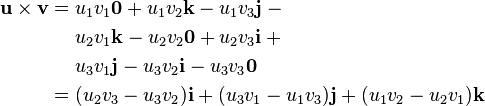
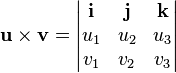
Cross product as vector quantity
Let's learn Cross product because it's having huge application in physics to find moment of a force that is also called Torque defined as vector(r)cross*vector(F)=Torque which is a vector quantity having magnitude and direction.
So if you have been given two vectors a and b. then
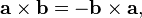
vec(a)crossvec(b)=a*b*sin(angle between a and b)n, Where n is a unit vector orthogonal to both vector a and b ,as curl is taken anti clockwise direction as shown graphically
.
The cross product a × b is defined as a vector c that is perpendicular to both a and b, with a direction given by the right-hand rule and a magnitude equal to the area of the parallelogram that the vectors span.
The cross product is defined by the formula

By convention, the direction of the vector n is given by the right-hand rule, where one simply points the forefinger of the right hand in the direction of a and the middle finger in the direction of b. Then, the vector n is coming out of the thumb (see the picture on the right). Using this rule implies that the cross-product is anti-commutative, i.e., b × a = −(a × b). By pointing the forefinger toward b first, and then pointing the middle finger toward a, the thumb will be forced in the opposite direction, reversing the sign of the product vector.
Using the cross product requires the handedness of the coordinate system to be taken into account (as explicit in the definition above). If a left-handed coordinate system is used, the direction of the vector n is given by the left-hand rule and points in the opposite direction.This, however, creates a problem because transforming from one arbitrary reference system to another (e.g., a mirror image transformation from a right-handed to a left-handed coordinate system), should not change the direction of n.

In 1881, Josiah Willard Gibbs, and independently Oliver Heaviside, introduced both the dot product and the cross product using a period (a . b) and an "x" (a x b), respectively, to denote them.
In 1877, to emphasize the fact that the result of a dot product is a scalar while the result of a cross product is a vector, William Kingdon Clifford coined the alternative names scalar product and vector product for the two operations. These alternative names are still widely used in the literature.Both the cross notation (a × b) and the name cross product were possibly inspired by the fact that each scalar component of a × b is computed by multiplying non-corresponding components of a and b. Conversely, a dot product a · b involves multiplications between corresponding components of a and b. As explained below, the cross product can be expressed in the form of a determinant of a special 3×3 matrix. According to Sarrus' rule, this involves multiplications between matrix elements identified by crossed diagonals.
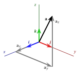
The standard basis vectors i, j, and k satisfy the following equalities:
These equalities, together with the distributivity and linearity of the cross product (but both do not follow easily from the definition given above), are sufficient to determine the cross product of any two vectors u and v. Each vector can be defined as the sum of three orthogonal components parallel to the standard basis vectors:

The cross product can also be expressed as


The magnitude of the cross product can be interpreted as the positive area of the parallelogram having a and b as sides
Unit vectors enable two convenient identities: the dot product of two unit vectors yields the cosine (which may be positive or negative) of the angle between the two unit vectors. The magnitude of the cross product of the two unit vectors yields the sine (which will always be positive).
g that is only possible if b − c = 0 so they are identical.
 is a 3-by-3 matrix and
  is the transpose of the inverse. It can be readily seen how this formula reduces to the former one if is a rotation matrix.
Another identity relates the cross product to the scalar triple product:
The combination of this requirement and the property that the cross product be orthogonal to its constituents a and b provides an alternative definition of the cross product.
It is a special case of another formula, also sometimes called Lagrange's identity, which is the three dimensional case of the Binet-Cauchy identity:
The cross product occurs in the formula for the vector operator curl. It is also used to describe the Lorentz force experienced by a moving electrical charge in a magnetic field. The definitions of torque and angular momentum also involve the cross product.
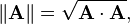
Dot product:A dot product between two vectors is a scalar quantity only having magnitude.It has a huge application in Linear Algebra which i am going discuss today.In Linear Algebra we define the dot product between a row vector and a column vector as a matrix multiplication ,Thus Dot product in Linear Algebra is matrix Multiplication of row and column matrix representing the x,y,z component of vectors as the element of matrix as shown diagramatically

 In three-dimensional space, the dot product contrasts with the cross product of two vectors, which produces a pseudovector
as the result. The dot product is directly related to the cosine of the
angle between two vectors in Euclidean space of any number of
dimensions.
In three-dimensional space, the dot product contrasts with the cross product of two vectors, which produces a pseudovector
as the result. The dot product is directly related to the cosine of the
angle between two vectors in Euclidean space of any number of
dimensions.
Definition of dot product:
The dot product is often defined in one of two ways: algebraically or geometrically. The geometric definition is based on the notions of angle and distance (magnitude of vectors). The equivalence of these two definitions relies on having a Cartesian coordinate system for Euclidean space.
In modern presentations of Euclidean geometry, the points of space are defined in terms of their Cartesian coordinates, and Euclidean space itself is commonly identified with the real coordinate space Rn. In such a presentation, the notions of length and angles are not primitive. They are defined by means of the dot product: the length of a vector is defined as the square root of the dot product of the vector by itself, and the cosine of the (non oriented) angle of two vectors of length one is defined as their dot product. So the equivalence of the two definitions of the dot product is a part of the equivalence of the classical and the modern formulations of Euclidean geometry.
Velocity in a Plane:
To describe the motion of an object in a plane, we first need to be able to describe the object’s position Often, it’s useful to use a familiar x-y axis system as shown in the Figure
For example, when a football player kicks a field goal, the ball (represented by point P) moves in a vertical plane. The ball’s
horizontal distance from the origin O at any time is x, and its vertical distance above the ground at any time is y. The numbers x and and y are called the coordinates of point P.The vector r from the origin O to point P is called the position vector of point P, and the Cartesian coordinates x and y of point P are the x and y components, respectively, of vector r.The distance of point P from the origin is the magnitude of vector r
The polar coordinates r and ϕ can be converted to the Cartesian coordinates x and y by using the trigonometric functions sine and cosine:


 (as in the Pythagorean theorem or the Euclidean norm), and
 ,
,
Let's consider a particle in this polar or Cartesian Coordinate system is at point P1 and moves to P2 as shown in the following figure
Let's understand the concept of Average velocity: Above figure in pink shows us that.
So what if we want to find the velocity at a particular instant of time to understand this we require to understand the concept of differential calculus:
The concept of instantaneous velocity and the differential calculus.
To understand instantaneous velocity ie the velocity at a point in the path of motion we require to understand the slope of tangent to the curve at that point .To understand the concept of slope of a tangent to a curve we have to understand Derivative of a function at any poin P(x,y) .And To understand Derivative of a function we require to understand a branch of differential calculus called Limit of a function means approximate value of a function when Domain X-->a, Where a must lie within domain and we write it mathematically as a (-Domain .
We define the instantaneous velocity as follows:
At every point along the path, the instantaneous velocity vector is
tangent to the path.
Because velocity is a vector quantity, we may represent it either in terms of its components or in terms of its magnitude and direction,
The direction of an object’s instantaneous velocity at any point is always tangent to the path at that point. But in general, the position vector r does not have the same direction as the instantaneous velocity v (The direction of the position vector r depends on where you place the origin, while the direction of is determined by the shape of the path.)
Acceleration in a Plane:
Observe the figure given below
Average acceleration is a vector quantity in the same direction as the vector, we stressed that acceleration is a quantitative description of the dv.
Again to understand the concept of instantaneous acceleration we require to apply the concept of Limit from differential calculus.
Let's understand instantaneous acceleration:
The instantaneous acceleration vector at point P1 as shown in the above figure does not have the same direction as the instantaneous velocity vector V at that point in general,there is no reason it should. ( The velocity and acceleration components of a particle moving along a line could have opposite signs also.)The construction in above Figure shows that the acceleration vector must always point toward the concave side of the curved path. When a particle moves in a curved path, it always has nonzero acceleration, even when it moves with constant speed. More generally, acceleration is associated with change of speed change of direction of velocity, or both.
We often represent the acceleration of a particle in terms of the components of this vector quantity.
Two special cases a) acceleration parallel to object's velocity
b)acceleration orthogonal to object's velocity
Cross product as vector quantity
Let's learn Cross product because it's having huge application in physics to find moment of a force that is also called Torque defined as vector(r)cross*vector(F)=Torque which is a vector quantity having magnitude and direction.
So if you have been given two vectors a and b. then
vec(a)crossvec(b)=a*b*sin(angle between a and b)n, Where n is a unit vector orthogonal to both vector a and b ,as curl is taken anti clockwise direction as shown graphically
.

Finding the direction of the cross product by the right-hand rule
The cross product of two vectors a and b is defined only in three-dimensional space and is denoted by a × b. In physics, sometimes the notation a ∧ b is used, though this is avoided in mathematics to avoid confusion with the exterior product.The cross product a × b is defined as a vector c that is perpendicular to both a and b, with a direction given by the right-hand rule and a magnitude equal to the area of the parallelogram that the vectors span.
The cross product is defined by the formula


The cross product a × b (vertical, in purple) changes as the angle between the vectors a (blue) and b (red) changes. The cross product is always perpendicular to both vectors, and has magnitude zero when the vectors are parallel and maximum magnitude ‖a‖‖b‖ when they are perpendicular.
Using the cross product requires the handedness of the coordinate system to be taken into account (as explicit in the definition above). If a left-handed coordinate system is used, the direction of the vector n is given by the left-hand rule and points in the opposite direction.This, however, creates a problem because transforming from one arbitrary reference system to another (e.g., a mirror image transformation from a right-handed to a left-handed coordinate system), should not change the direction of n.

According to Sarrus' rule, the determinant of a 3×3 matrix involves multiplications between matrix elements identified by crossed diagonals
In 1877, to emphasize the fact that the result of a dot product is a scalar while the result of a cross product is a vector, William Kingdon Clifford coined the alternative names scalar product and vector product for the two operations. These alternative names are still widely used in the literature.Both the cross notation (a × b) and the name cross product were possibly inspired by the fact that each scalar component of a × b is computed by multiplying non-corresponding components of a and b. Conversely, a dot product a · b involves multiplications between corresponding components of a and b. As explained below, the cross product can be expressed in the form of a determinant of a special 3×3 matrix. According to Sarrus' rule, this involves multiplications between matrix elements identified by crossed diagonals.
Computing the cross product

Standard basis vectors (i, j, k, also denoted e1, e2, e3) and vector components of a (ax, ay, az, also denoted a1, a2, a3)


These equalities, together with the distributivity and linearity of the cross product (but both do not follow easily from the definition given above), are sufficient to determine the cross product of any two vectors u and v. Each vector can be defined as the sum of three orthogonal components parallel to the standard basis vectors:


Matrix notation

Use of Sarrus' rule to find the cross product of u and v


Geometric meaning of Cross product says that it has direction hence it is a vector.

Figure 1. The area of parallelogram as the magnitude of a cross product

Figure 2. Three vectors defining a parallelepiped


Unit vectors enable two convenient identities: the dot product of two unit vectors yields the cosine (which may be positive or negative) of the angle between the two unit vectors. The magnitude of the cross product of the two unit vectors yields the sine (which will always be positive).
Algebraic properties

- If the cross product of two vectors is the zero vector (i.e. a × b = 0), then either one or both of the inputs is the zero vector, (a = 0 and/or b = 0) or else they are parallel or antiparallel (a ∥ b) so that the sine of the angle between them is zero (θ = 0° or θ = 180° and sinθ = 0).
- The self cross product of a vector is the zero vector, i.e., a × a = 0.
- The cross product is anticommutative,
- distributive over addition,

- and compatible with scalar multiplication so that

- It is not associative, but satisfies the Jacobi identity:

- The cross product does not obey the cancellation law: that is, a × b = a × c with a ≠ 0 does not imply b = c, but only that:
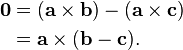

g that is only possible if b − c = 0 so they are identical.
- If a · b = a · c and a × b = a × c, for non-zero vector a, then b = c, as
 and
and
- From the geometrical definition, the cross product is invariant under rotations about the axis defined by a × b. In formulae:
 , with
  rotation matrix.
 , with
  rotation matrix.
 is a 3-by-3 matrix and
  is the transpose of the inverse. It can be readily seen how this formula reduces to the former one if is a rotation matrix.
- The cross product of two vectors lies in the null space of the 2×3 matrix with the vectors as rows:

- For the sum of two cross products, the following identity holds:

Differentiation of Cross product of vectors
Main article: Vector-valued function § Derivative and vector multiplication
The product rule applies to the cross product in a similar manner:
Triple product expansion.
Triple product
The cross product is used in both forms of the triple product. The scalar triple product of three vectors is defined as


Another identity relates the cross product to the scalar triple product:

Alternative formulation
The cross product and the dot product are related by:


The combination of this requirement and the property that the cross product be orthogonal to its constituents a and b provides an alternative definition of the cross product.
Lagrange's identity
The relation:


It is a special case of another formula, also sometimes called Lagrange's identity, which is the three dimensional case of the Binet-Cauchy identity:

The cross product occurs in the formula for the vector operator curl. It is also used to describe the Lorentz force experienced by a moving electrical charge in a magnetic field. The definitions of torque and angular momentum also involve the cross product.
Dot product:A dot product between two vectors is a scalar quantity only having magnitude.It has a huge application in Linear Algebra which i am going discuss today.In Linear Algebra we define the dot product between a row vector and a column vector as a matrix multiplication ,Thus Dot product in Linear Algebra is matrix Multiplication of row and column matrix representing the x,y,z component of vectors as the element of matrix as shown diagramatically
Definition of dot product:
The dot product is often defined in one of two ways: algebraically or geometrically. The geometric definition is based on the notions of angle and distance (magnitude of vectors). The equivalence of these two definitions relies on having a Cartesian coordinate system for Euclidean space.
In modern presentations of Euclidean geometry, the points of space are defined in terms of their Cartesian coordinates, and Euclidean space itself is commonly identified with the real coordinate space Rn. In such a presentation, the notions of length and angles are not primitive. They are defined by means of the dot product: the length of a vector is defined as the square root of the dot product of the vector by itself, and the cosine of the (non oriented) angle of two vectors of length one is defined as their dot product. So the equivalence of the two definitions of the dot product is a part of the equivalence of the classical and the modern formulations of Euclidean geometry.
Algebraic definition
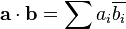
The dot product of two vectors A = [A1, A2, ..., An] and B = [B1, B2, ..., Bn] is defined as:
![\begin{align}
\ [1, 3, -5] \cdot [4, -2, -1] &= (1)(4) + (3)(-2) + (-5)(-1) \\
&= 4 - 6 + 5 \\
&= 3.
\end{align}](http://upload.wikimedia.org/math/1/3/1/131c946a85f1e689a920763c11f89d5a.png)
Geometric definition or Vector Algebra definition
In Euclidean space, a Euclidean vector is a geometrical object that possesses both a magnitude and a direction. A vector can be pictured as an arrow. Its magnitude is its length, and its direction is the direction that the arrow points. The magnitude of a vector A is denoted by
 . The dot product of two Euclidean vectors A and B is defined by[
In particular, if A and B are orthogonal, then the angle between them is 90° and


Scalar projection and first properties:
The scalar projection (or scalar component) of a Euclidean vector A in the direction of a Euclidean vector B is given by

In terms of the geometric definition of the dot product, this can be rewritten

 is the unit vector in the direction of B
Cosine Rule in Trigonometry is related to Dot product of vectors means that using dot product we can derive Cosine rule of trigonometry as follows
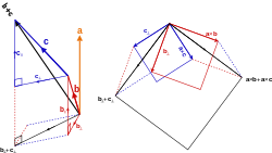
Given two vectors a and b separated by angle θ (see image right), they form a triangle with a third side c = a − b. The dot product of this with itself is:

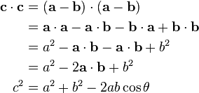
This is an application of dot product to derive Cosine law it can also be used to derive parallelogram law of vector addition.
In physics, vector magnitude is a scalar in the physical sense, i.e. a physical quantity independent of the coordinate system, expressed as the product of a numerical value and a physical unit, not just a number. The dot product is also a scalar in this sense, given by the formula, independent of the coordinate system. Examples include:
- Mechanical work is the dot product of force and displacement vectors.
- Magnetic flux is the dot product of the magnetic field and the area vectors.
Mechanical work in physics:
For moving objects, the quantity of work/time (power) is calculated. Thus, at any instant, the rate of the work done by a force (measured in joules/second, or watts) is the scalar product of the force (a vector), and the velocity vector of the point of application. This scalar product of force and velocity is classified as instantaneous power. Just as velocities may be integrated over time to obtain a total distance, by the fundamental theorem of calculus, the total work along a path is similarly the time-integral of instantaneous power applied along the trajectory of the point of application.
Application of Dot Product in calculating Work done
Work is the result of a force on a point that moves through a distance. As the point moves, it follows a curve X, with a velocity v, at each instant. The small amount of work δW that occurs over an instant of time dt is calculated as


If the force is always directed along this line, and the magnitude of the force is F, then this integral simplifies to


This calculation can be generalized for a constant force that is not directed along the line, followed by the particle. In this case the dot product F·ds = Fcosθds, where θ is the angle between the force vector and the direction of movement,[that is

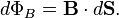
Magnetic flux :It can calculated using Magnetic field density vector B dot with differential Area vector dS summed over all differential area vector over the surface as  Let's see it in greater detail because it will be useful to calculate flux associated with any vector field F over any surface area S as following:
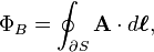
In physics, specifically electromagnetism, the magnetic flux (often denoted Φ or ΦB) through a surface is the surface integral of the normal component of the magnetic field B passing through that surface. The SI unit of magnetic flux is the weber (Wb) (in derived units: volt-seconds), and the CGS unit is the maxwell. Magnetic flux is usually measured with a fluxmeter, which contains measuring coils and electronics, that evaluates the change of voltage in the measuring coils to calculate the magnetic flux.
he magnetic interaction is described in terms of a vector field, where each point in space (and time) is associated with a vector that determines what force a moving charge would experience at that point (search Lorentz force). Since a vector field is quite difficult to visualize at first, in elementary physics one may instead visualize this field with field lines. The magnetic flux through some surface, in this simplified picture, is proportional to the number of field lines passing through that surface (in some contexts, the flux may be defined to be precisely the number of field lines passing through that surface; although technically misleading, this distinction is not important). Note that the magnetic flux is the net number of field lines passing through that surface; that is, the number passing through in one direction minus the number passing through in the other direction (see below for deciding in which direction the field lines carry a positive sign and in which they carry a negative sign). In more advanced physics, the field line analogy is dropped and the magnetic flux is properly defined as the surface integral of the normal component of the magnetic field passing through a surface. If the magnetic field is constant, the magnetic flux passing through a surface of vector area S is:
magnetic flux passing through a surface of vector area S is
Let's see it in greater detail because it will be useful to calculate flux associated with any vector field F over any surface area S as following:In physics, specifically electromagnetism, the magnetic flux (often denoted Φ or ΦB) through a surface is the surface integral of the normal component of the magnetic field B passing through that surface. The SI unit of magnetic flux is the weber (Wb) (in derived units: volt-seconds), and the CGS unit is the maxwell. Magnetic flux is usually measured with a fluxmeter, which contains measuring coils and electronics, that evaluates the change of voltage in the measuring coils to calculate the magnetic flux.
he magnetic interaction is described in terms of a vector field, where each point in space (and time) is associated with a vector that determines what force a moving charge would experience at that point (search Lorentz force). Since a vector field is quite difficult to visualize at first, in elementary physics one may instead visualize this field with field lines. The magnetic flux through some surface, in this simplified picture, is proportional to the number of field lines passing through that surface (in some contexts, the flux may be defined to be precisely the number of field lines passing through that surface; although technically misleading, this distinction is not important). Note that the magnetic flux is the net number of field lines passing through that surface; that is, the number passing through in one direction minus the number passing through in the other direction (see below for deciding in which direction the field lines carry a positive sign and in which they carry a negative sign). In more advanced physics, the field line analogy is dropped and the magnetic flux is properly defined as the surface integral of the normal component of the magnetic field passing through a surface. If the magnetic field is constant, the magnetic flux passing through a surface of vector area S is:
magnetic flux passing through a surface of vector area S is


Above derivation can be assisted by following figure


Projection of dS.n along yellow vector= (dS.n)*cos(theta)
Above Derivation using above figure in slightly different manner!
Magnetic flux through a closed surface an application of Dot Product:
Gauss's law for magnetism, which is one of the four Maxwell's equations, states that the total magnetic flux through a closed surface is equal to zero. (A "closed surface" is a surface that completely encloses a volume(s) with no holes.) This law is a consequence of the empirical observation that magnetic monopoles have never been found.In other words, Gauss's law for magnetism is the statement:


Magnetic flux through an open surface an application of Dot Product:
While the magnetic flux through a closed surface is always zero, the magnetic flux through an open surface need not be zero and is an important quantity in electromagnetism. For example, a change in the magnetic flux passing through a loop of conductive wire will cause an electromotive force, and therefore an electric current, in the loop. The relationship is given by Faraday's law: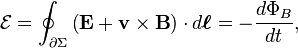
 is the electromotive force (EMF),
- ΦB is the magnetic flux through the open surface Σ,
- ∂Σ is the boundary of the open surface Σ; note that the surface, in general, may be in motion and deforming, and so is generally a function of time. The electromotive force is induced along this boundary.
- dℓ is an infinitesimal vector element of the contour ∂Σ,
- v is the velocity of the boundary ∂Σ,
- E is the electric field,
- B is the magnetic field.
For an open surface Σ, the electromotive force
 along the surface boundary, ∂Σ, is a combination of the boundary's motion, with velocity v, through a magnetic field B (illustrated by the generic F field in the diagram) and the induced electric field caused by the changing magnetic field.
electric flux calculation :
By way of contrast, Gauss's law for electric fields, another of Maxwell's equations, is

- E is the electric field,
- S is any closed surface,
- Q is the total electric charge inside the surface S,
- ε0 is the electric constant (a universal constant, also called the "permittivity of free space").
So dot product has a huge application in both physics and different domain of mathematics i will come with more application in physics today let's come to mathematics complex domain.
Complex vectors and application of dot product:
Before understanding dot product in Complex number, let's understand complex number first:
Complex numbers:
Every complex number can be represented as a point in the complex plane, and can therefore be expressed by specifying either the point's Cartesian coordinates (called rectangular or Cartesian form) or the point's polar coordinates (called polar form). The complex number z can be represented in rectangular form as can well be mapped onto Cartesian Coordinate System as shown below
- also in polar form as shown below
 and this can be represented onto polar coordinate system as shown below here

Polar form of complex number
 We can write any complex number
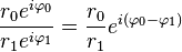
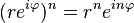
For the operations of multiplication, division, and exponentiation of complex numbers, it is generally much simpler to work with complex numbers expressed in polar form rather than rectangular form. From the laws of exponentiation:
- Multiplication:

- Division:
- Exponentiation (De Moivre's formula):
Come to application of Dot Product in Complex number
For vectors with complex entries, using the given definition of the dot product would lead to quite different properties. For instance the dot product of a vector with itself would be an arbitrary complex number, and could be zero without the vector being the zero vector (such vectors are called isotropic); this in turn would have consequences for notions like length and angle. Properties such as the positive-definite norm can be salvaged at the cost of giving up the symmetric and bilinear properties of the scalar product, through the alternative definition


Another application of dot product in mathematics is Inner Products :The inner product generalizes the dot product to abstract vector spaces over a field of scalars, being either the field of real numbers
 or the field of complex numbers
  . It is usually denoted by
  . The inner product of two vectors over the field of complex numbers is, in general, a complex number, and is sesquilinear instead of bilinear. An inner product space is a normed vector space, and the inner product of a vector with itself is real and positive-definite.
Application of Dot Product in the projection of one function onto another function:
Dot product for projection of function onto another function
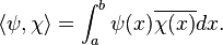
The dot product is defined for vectors that have a finite number of entries. Thus these vectors can be regarded as discrete functions: a length-n vector u is, then, a function with domain {k ∈ ℕ ∣ 1 ≤ k ≤ n}, and ui is a notation for the image of i by the function/vector u.This notion can be generalized to continuous functions: just as the inner product on vectors uses a sum over corresponding components, the inner product on functions is defined as an integral over some interval a ≤ x ≤ b (also denoted [a, b]):

In my next paper i will come with the more application of Dot product in Physics and Image compression and problems in physics based on Dot product.
Problems based on vector calculus :
Electronics And communication by Md Tauseef Ibrahim/Abraham Malik
Search the related topics like the Algebra of vector and its Dynamics from http://t.co/eQSpd40fb2 the physics,nature pic.twitter.com/YNt3BVSv6u
— Abraham Malik (@brhmmlk93_malik) March 4, 2015
https://t.co/vcjSU1HzdO
y=Cos(x) and Inverse of Cosine as x=arccos(y),but plotted in Cartesian system as X->y &y->X pic.twitter.com/rjL1ctkuvb
— Abraham Malik (@brhmmlk93_malik) March 6, 2015
No comments:
Post a Comment